KLT Algorithm - Concept and Implementation Procedure

KLT is a combined feature detection and tracking technique. It was first presented in 1981 by Lucas and Kanade and was extensively enhanced by Shi and Tomasi (1994). Over three decades, the algorithm has been widely used in a variety of applications ranging from eye tracking to military surveillance activities. Since the technique is well-known for its computational efficiency, it has often been applied in real-time applications.

1. Feature Detection

KLT needs to detect features to serve as tie-points between one image and the next. The KLT feature detection algorithm was proposed by Shi and Tomasi (1994). The underlying concept of the algorithm is based on the work of Harris and Stephens (1988) with some slight changes in the definition of “good” features. Harris and Stephens (1988) start by determining the autocorrelation matrix, G, for each pixel in the image as Eq. (2.1).

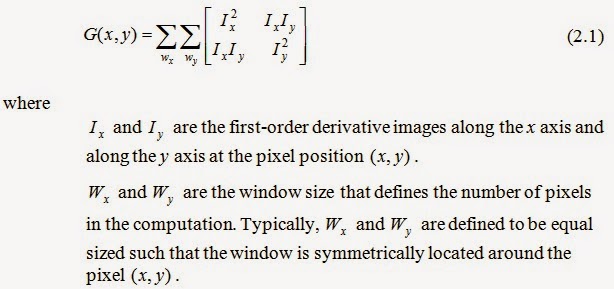
A corner by definition of Harris and Stephens is a position in the image where its autocorrelation matrix, presented Eq. (2.1) has two large eigenvalues (Bradski and Kaehler, 2008). This implies that there are edges in at least two separate directions around the point which corresponds to a real corner. Based on a basic fact that the determinant of a matrix with eigenvalues Lamda1 and Lamda2 is the product Lamda1*Lamda2 and the trace is Lamda1+Lamda2(Langer, 2012), a point is defined as a corner if Eq. (2.2) holds.

Shi and Tomasi (1994) later demonstrated that a good corner results when the smaller value of the two eigenvalues is sufficiently large. Let Lamda_m be defined as Eq. (2.3). Thus, the definition of a good corner by Shi and Tomasi is presented as Eq. (2.4). Their approach is not only comparable to but, in many cases, shows more satisfactory results than Harris’s method (Bradski and Kaehler, 2008).

A large value of threshold T produces a large number of features but can degrade their quality. In contrast, a low value of the threshold restricts the number of features such that it produces a small number of highly salient features. Since the selection of an appropriate threshold is crucial, many implementations derive this value from the largest minimum eigenvalue observed in the image. In the OpenCV implementation, as an example, this cutoff threshold is defined as the product the largest minimum-eigenvalue and the input parameter qualityLevel, denoted as r where r=[0..1] (Bradski and Kaehler, 2008; OpenCV, 2010). The KLT feature extraction procedure is summarized as the figure below.

2. Feature Tracking

The most common definition of Optical Flow was proposed by Horn (1986). He described optical flow as the apparent motion of brightness patterns in an image sequence. This apparent motion may be due to moving objects in the scene, or the motion of the camera, or even external sources such as light change (Black, 1992; Negahdaripour, 1998). Referring to the figure below, suppose a point p on an image frame captured at time t has coordinates (x,y). In the next frame acquired at time t+dt, the point p is present at coordinates (x+dx,y+dy).

Optical flow may be classified into two categories: dense optical flow and sparse optical flow. Dense optical flow (often referred to as velocity) refers to displacements associated with each and every pixel in an image, such that this presents a velocity field. Since dense optical flow considers motion associated with every pixel, it involves high computational cost. Calculating this type of optical flow may require interpolation techniques to deduce optical flow associated with pixels that are difficult to track, such as the motion of a white sheet of paper (Bradski and Kaehler, 2008).

As opposed to dense optical flow, sparse optical flow refers to the motions of some specific pixels. These pixels are usually features that are easy to identify such as corners. Since it deals with a limited number of features, the latter technique is more computationally efficient. It has been shown that dense optical flow calculation techniques cannot handle large displacements between frames, which are typical in aerial images. Examples of dense optical flow and sparse optical flow presented on real images are illustrated below. The KLT tracking technique is classified as a sparse tracking approach.

The KLT tracker was first introduced by Lucas and Kanade in 1981 and is often referred to as the Lucas-Kanade or LK algorithm. As summarized by Bradski and Kaehler (2008), the algorithm relies on three basic assumptions as described below.

1. Brightness constancy. The brightness of a pixel does not change from frame to frame. Thus a pixel can be located in the subsequent frame based on its brightness value since I( x(t), t ) = I( x(t+dt), t+dt ). As a result, Eq. (2.7) holds.

2. Temporal persistence. The motion between frames is small and thus an object does not move much over time. Based on the brightness constancy, we can derive Eq. (2.8).

3.Spatial coherence. Neighboring pixels have similar motion.

The goal of the KLT tracker is to minimize the sum of squared error between the template T(x) and the image J(x) (Lucas and Kanade 1981; Baker and Matthews, 2004). The mentioned error is the intensity difference e between these two images computed over the area of the template A centered at the position x where x=[x y]T. The dissimilarity function can be calculated as Eq. (2.9).

where W(x;p) is a warping function in which p is the set of warping parameters. The warping function W maps each vector x in the template window A to a new position (usually at sub-pixel level) in the image J using the transformation parameters p (Glasbey and Mardia, 1998). The warping function used in the Lucas-Kanade algorithm, presented as Eq. (2.10), is known as a translation model, which aims to compute the optical flow vector d = (dx,dy).

Eq. (2.9) is a non-linear problem and can be solved through the least square optimization approach. Lucas and Kanade (1981) assume a starting point p is known, and thus Eq. (2.9) can be re-written as Eq. (2.11). Therefore, the problem becomes that of solving for an increment vector Δp. Lucas and Kanade (1981) solves this least square optimization problem by modifying p as p+Δp -> p, iteratively through the Newton-Raphson scheme such that Eq. (2.11) is minimized or Δp is below the threshold Epsilon. This is illustrated as the figure below.

Given that,

The content presented here is adopt from
Tanathong, S., 2013. Fast Image Matching for Real-time Georeferencing Using Exterior Orientation Observed from GPS/INS. Ph.D. Dissertation, the University of Seoul, Seoul, Korea.