The package comes with both intrinsic and extrinsic calibration for multi-camera system. The advantage of this technique is that it does not require overlapping fields of view between cameras. In order to determine the scale metric between cameras, it requires odometry data which can be from the wheel or GPS/IMU system. The package is developed in C++ on the Ubuntu platform. I attempted to port it to Windows but due to its dependency, it is a complicated task. An easy solution is to use CamOdoCal is to install Ubuntu on Oracle Virtual Box (https://www.virtualbox.org/) on my Windows machine, and this works for me to compile and use it.
Reference:
Heng, L., Li, B., Pollefeys, M., 2013. CamOdoCal: Automatic intrinsic and extrinsic calibration of a rig with multiple generic cameras and odometry.
Link:
https://github.com/hengli/camodocal
http://people.inf.ethz.ch/hengli/camodocal/
To be updated ..
Thursday, June 9, 2016
Thursday, August 28, 2014
My very first start with RaspberryPi
I have just received my first RaspberryPi early this week. The one I have is Raspberry Pi with model B+.

A quick starting guide for RaspberryPi can be found at http://www.raspberrypi.org/help/quick-start-guide/.
Luckily for me that I have a chance to attend a free training course conducted by Deaware supported by SIPA. It helps me understand RaspberryPi quickly.
The RaspberryPi with Model B+ has the following specifications:
* 40-pin GPIO header.
* 4 USB ports.
* Micro SD card socket.
The figure below presents the high-level design of the Model B+. (Picture from http://www.raspberrypi.org/product/model-b-plus/)

And, the GPIO diagram is presented below: (Picture from http://www.raspberrypi.org/product/model-b-plus/)

The devices required for my RaspberryPi project are:
1. Raspberry Pi
2. A micro USB cable for supplying power to the RaspberryPi
3. A LAN cable RJ45
4. SD card at least 4GB for OS, libraries and programs to work with the RaspberryPi

The operating system I have installed for my RaspberyPi is Raspbian (Raspbian.org). Its image can be download directly from http://www.raspberrypi.org/downloads/

After the image is loaded, extract the zip file and have our image file with extension .img. We can then write the image of Raspbian OS to the SD card which later will be put into the RaspberryPi SD socket. To burn the image using a computer with Windows OS, follow the instruction here.
1. Insert the SD card into the SD card reader on our computer.
2. Write the image of Raspbian into the SD card using Win32DiskImager, which can be download from http://sourceforge.net/projects/win32diskimager/.
3. Right click on the Win32DiskImager.EXE and select Run as Administrator.
4. On the Win32DiskImager program, browse to the image file from our Step 2 and make sure that the drive to the SD card is correct.
5. Then click Write.

After this point, we have Raspbian OS ready for our RaspberryPi. Since the image written into the SD card is about 2.7GB, it makes the capacity of the SD card to be the same as that size. We later have to expand the size of our SD card to be back to its original capacity. This configuration change must be done at the OS of the RaspberryPi. Therefore, we will not put the SD card into the RaspberryPi board yet. What we are gonna do now is to make our computer be able to communicate with the RaspberryPi.
We are gonna make our computer talk to the Pi via network (LAN cable). To do so, we assign a static IP address to our computer manually and we will assign one to our RaspberryPi, in which these two IP address must be in the same network. For example, our computer has IP: 192.168.10.10 and our Pi has IP: 192.10.10.20.

For Windows, we can simply set IP on our computer by going to Control Panel --> Network and Sharing Center --> Change adapter Settings. Then, right click at an Ethernet connection --> Properties --> Internet Protocol Version 4 --> Properties. After that assign an IP address for our computer to talk with our Pi.

To set an IP address for our Pi device, we make change the file named cmdline.txt in the SD card.

Edit the file cmdline.txt by adding
ip=192.168.10.20
at the end of the line. Make sure that the added IP address is on the same line.

What we are doing next is to eject the SD card from our computer and put the SD card into its slot on the RaspberryPi board at the back side, as shown in the picture below.

Connect our RaspberryPi board with our computer with LAN cable and supply power to the board using the USB cable. Now, we are ready to start our RaspberryPi.

We can test our connection with Pi by pinging to the Pi's IP address.
ping 192.168.10.20
And, we should find our Pi.

Once we found our Pi, we can control the Pi by remotely accessing the Pi's console.
Here, we use mRemoteNG to access the Pi's console. mRemoteNG can be downloaded from http://www.mremoteng.org/download. What we have to do is to create a new connection to the RaspberryPi with our defined IP (192.168.10.20).
The default user name and password for the RaspberryPi is
User: pi
Password: raspberry

Connect and now we can access the Pi's console.

On the console, we use the first command to check the size of the SD card. The second command is to config the RaspberryPi, in which we want to expand the size of the SD card.
df -h
sudo raspi-config
Here is the screen to expand the size of the SD card.

References:
Training material by Deaware.
www.raspberrypi.org
Thursday, August 21, 2014
KLT Algorithm - Concept and Implementation Procedure
KLT is a combined feature detection and tracking technique. It was first presented in 1981 by Lucas and Kanade and was extensively enhanced by Shi and Tomasi (1994). Over three decades, the algorithm has been widely used in a variety of applications ranging from eye tracking to military surveillance activities. Since the technique is well-known for its computational efficiency, it has often been applied in real-time applications.
1. Feature Detection
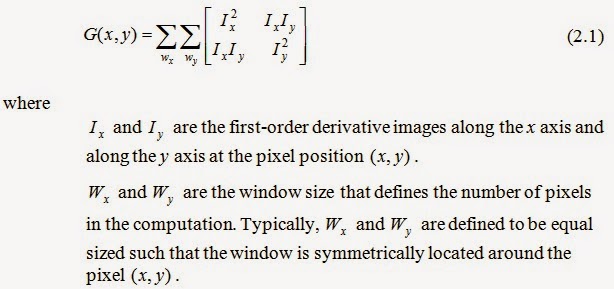
KLT needs to detect features to serve as tie-points between one image and the next. The KLT feature detection algorithm was proposed by Shi and Tomasi (1994). The underlying concept of the algorithm is based on the work of Harris and Stephens (1988) with some slight changes in the definition of “good” features. Harris and Stephens (1988) start by determining the autocorrelation matrix, G, for each pixel in the image as Eq. (2.1).

A corner by definition of Harris and Stephens is a position in the image where its autocorrelation matrix, presented Eq. (2.1) has two large eigenvalues (Bradski and Kaehler, 2008). This implies that there are edges in at least two separate directions around the point which corresponds to a real corner. Based on a basic fact that the determinant of a matrix with eigenvalues Lamda1 and Lamda2 is the product Lamda1*Lamda2 and the trace is Lamda1+Lamda2(Langer, 2012), a point is defined as a corner if Eq. (2.2) holds.

Shi and Tomasi (1994) later demonstrated that a good corner results when the smaller value of the two eigenvalues is sufficiently large. Let Lamda_m be defined as Eq. (2.3). Thus, the definition of a good corner by Shi and Tomasi is presented as Eq. (2.4). Their approach is not only comparable to but, in many cases, shows more satisfactory results than Harris’s method (Bradski and Kaehler, 2008).

A large value of threshold T produces a large number of features but can degrade their quality. In contrast, a low value of the threshold restricts the number of features such that it produces a small number of highly salient features. Since the selection of an appropriate threshold is crucial, many implementations derive this value from the largest minimum eigenvalue observed in the image. In the OpenCV implementation, as an example, this cutoff threshold is defined as the product the largest minimum-eigenvalue and the input parameter qualityLevel, denoted as r where r=[0..1] (Bradski and Kaehler, 2008; OpenCV, 2010). The KLT feature extraction procedure is summarized as the figure below.

2. Feature Tracking
The most common definition of Optical Flow was proposed by Horn (1986). He described optical flow as the apparent motion of brightness patterns in an image sequence. This apparent motion may be due to moving objects in the scene, or the motion of the camera, or even external sources such as light change (Black, 1992; Negahdaripour, 1998). Referring to the figure below, suppose a point p on an image frame captured at time t has coordinates (x,y). In the next frame acquired at time t+dt, the point p is present at coordinates (x+dx,y+dy).

Optical flow may be classified into two categories: dense optical flow and sparse optical flow. Dense optical flow (often referred to as velocity) refers to displacements associated with each and every pixel in an image, such that this presents a velocity field. Since dense optical flow considers motion associated with every pixel, it involves high computational cost. Calculating this type of optical flow may require interpolation techniques to deduce optical flow associated with pixels that are difficult to track, such as the motion of a white sheet of paper (Bradski and Kaehler, 2008).
As opposed to dense optical flow, sparse optical flow refers to the motions of some specific pixels. These pixels are usually features that are easy to identify such as corners. Since it deals with a limited number of features, the latter technique is more computationally efficient. It has been shown that dense optical flow calculation techniques cannot handle large displacements between frames, which are typical in aerial images. Examples of dense optical flow and sparse optical flow presented on real images are illustrated below. The KLT tracking technique is classified as a sparse tracking approach.

The KLT tracker was first introduced by Lucas and Kanade in 1981 and is often referred to as the Lucas-Kanade or LK algorithm. As summarized by Bradski and Kaehler (2008), the algorithm relies on three basic assumptions as described below.

1. Brightness constancy. The brightness of a pixel does not change from frame to frame. Thus a pixel can be located in the subsequent frame based on its brightness value since I( x(t), t ) = I( x(t+dt), t+dt ). As a result, Eq. (2.7) holds.
2. Temporal persistence. The motion between frames is small and thus an object does not move much over time. Based on the brightness constancy, we can derive Eq. (2.8).
3.Spatial coherence. Neighboring pixels have similar motion.

The goal of the KLT tracker is to minimize the sum of squared error between the template T(x) and the image J(x) (Lucas and Kanade 1981; Baker and Matthews, 2004). The mentioned error is the intensity difference e between these two images computed over the area of the template A centered at the position x where x=[x y]T. The dissimilarity function can be calculated as Eq. (2.9).
where W(x;p) is a warping function in which p is the set of warping parameters. The warping function W maps each vector x in the template window A to a new position (usually at sub-pixel level) in the image J using the transformation parameters p (Glasbey and Mardia, 1998). The warping function used in the Lucas-Kanade algorithm, presented as Eq. (2.10), is known as a translation model, which aims to compute the optical flow vector d = (dx,dy).

Eq. (2.9) is a non-linear problem and can be solved through the least square optimization approach. Lucas and Kanade (1981) assume a starting point p is known, and thus Eq. (2.9) can be re-written as Eq. (2.11). Therefore, the problem becomes that of solving for an increment vector Δp. Lucas and Kanade (1981) solves this least square optimization problem by modifying p as p+Δp -> p, iteratively through the Newton-Raphson scheme such that Eq. (2.11) is minimized or Δp is below the threshold Epsilon. This is illustrated as the figure below.

Given that,

The content presented here is adopt from
Tanathong, S., 2013. Fast Image Matching for Real-time Georeferencing Using Exterior Orientation Observed from GPS/INS. Ph.D. Dissertation, the University of Seoul, Seoul, Korea.
1. Feature Detection
KLT needs to detect features to serve as tie-points between one image and the next. The KLT feature detection algorithm was proposed by Shi and Tomasi (1994). The underlying concept of the algorithm is based on the work of Harris and Stephens (1988) with some slight changes in the definition of “good” features. Harris and Stephens (1988) start by determining the autocorrelation matrix, G, for each pixel in the image as Eq. (2.1).
A corner by definition of Harris and Stephens is a position in the image where its autocorrelation matrix, presented Eq. (2.1) has two large eigenvalues (Bradski and Kaehler, 2008). This implies that there are edges in at least two separate directions around the point which corresponds to a real corner. Based on a basic fact that the determinant of a matrix with eigenvalues Lamda1 and Lamda2 is the product Lamda1*Lamda2 and the trace is Lamda1+Lamda2(Langer, 2012), a point is defined as a corner if Eq. (2.2) holds.

Shi and Tomasi (1994) later demonstrated that a good corner results when the smaller value of the two eigenvalues is sufficiently large. Let Lamda_m be defined as Eq. (2.3). Thus, the definition of a good corner by Shi and Tomasi is presented as Eq. (2.4). Their approach is not only comparable to but, in many cases, shows more satisfactory results than Harris’s method (Bradski and Kaehler, 2008).

A large value of threshold T produces a large number of features but can degrade their quality. In contrast, a low value of the threshold restricts the number of features such that it produces a small number of highly salient features. Since the selection of an appropriate threshold is crucial, many implementations derive this value from the largest minimum eigenvalue observed in the image. In the OpenCV implementation, as an example, this cutoff threshold is defined as the product the largest minimum-eigenvalue and the input parameter qualityLevel, denoted as r where r=[0..1] (Bradski and Kaehler, 2008; OpenCV, 2010). The KLT feature extraction procedure is summarized as the figure below.

2. Feature Tracking
The most common definition of Optical Flow was proposed by Horn (1986). He described optical flow as the apparent motion of brightness patterns in an image sequence. This apparent motion may be due to moving objects in the scene, or the motion of the camera, or even external sources such as light change (Black, 1992; Negahdaripour, 1998). Referring to the figure below, suppose a point p on an image frame captured at time t has coordinates (x,y). In the next frame acquired at time t+dt, the point p is present at coordinates (x+dx,y+dy).

Optical flow may be classified into two categories: dense optical flow and sparse optical flow. Dense optical flow (often referred to as velocity) refers to displacements associated with each and every pixel in an image, such that this presents a velocity field. Since dense optical flow considers motion associated with every pixel, it involves high computational cost. Calculating this type of optical flow may require interpolation techniques to deduce optical flow associated with pixels that are difficult to track, such as the motion of a white sheet of paper (Bradski and Kaehler, 2008).
As opposed to dense optical flow, sparse optical flow refers to the motions of some specific pixels. These pixels are usually features that are easy to identify such as corners. Since it deals with a limited number of features, the latter technique is more computationally efficient. It has been shown that dense optical flow calculation techniques cannot handle large displacements between frames, which are typical in aerial images. Examples of dense optical flow and sparse optical flow presented on real images are illustrated below. The KLT tracking technique is classified as a sparse tracking approach.

The KLT tracker was first introduced by Lucas and Kanade in 1981 and is often referred to as the Lucas-Kanade or LK algorithm. As summarized by Bradski and Kaehler (2008), the algorithm relies on three basic assumptions as described below.

1. Brightness constancy. The brightness of a pixel does not change from frame to frame. Thus a pixel can be located in the subsequent frame based on its brightness value since I( x(t), t ) = I( x(t+dt), t+dt ). As a result, Eq. (2.7) holds.
2. Temporal persistence. The motion between frames is small and thus an object does not move much over time. Based on the brightness constancy, we can derive Eq. (2.8).
3.Spatial coherence. Neighboring pixels have similar motion.

The goal of the KLT tracker is to minimize the sum of squared error between the template T(x) and the image J(x) (Lucas and Kanade 1981; Baker and Matthews, 2004). The mentioned error is the intensity difference e between these two images computed over the area of the template A centered at the position x where x=[x y]T. The dissimilarity function can be calculated as Eq. (2.9).
where W(x;p) is a warping function in which p is the set of warping parameters. The warping function W maps each vector x in the template window A to a new position (usually at sub-pixel level) in the image J using the transformation parameters p (Glasbey and Mardia, 1998). The warping function used in the Lucas-Kanade algorithm, presented as Eq. (2.10), is known as a translation model, which aims to compute the optical flow vector d = (dx,dy).

Eq. (2.9) is a non-linear problem and can be solved through the least square optimization approach. Lucas and Kanade (1981) assume a starting point p is known, and thus Eq. (2.9) can be re-written as Eq. (2.11). Therefore, the problem becomes that of solving for an increment vector Δp. Lucas and Kanade (1981) solves this least square optimization problem by modifying p as p+Δp -> p, iteratively through the Newton-Raphson scheme such that Eq. (2.11) is minimized or Δp is below the threshold Epsilon. This is illustrated as the figure below.

Given that,

The content presented here is adopt from
Tanathong, S., 2013. Fast Image Matching for Real-time Georeferencing Using Exterior Orientation Observed from GPS/INS. Ph.D. Dissertation, the University of Seoul, Seoul, Korea.
CBits - a helper class to check/set in which images on an image sequence a (ground) point exists
A ground point (or an object point) may be captured or presented in multiple images in an image sequence if those images are overlapped. The figure below illustrates a ground point exists on multiple images.

For some situations, we need to know in which images a ground point exists. Aerial triangulation (AT) algorithm, for example, involves a large number of tiepoints, ground points, and EOs of all images in the sequence. Below is a picture of a file containing a list of tiepoints - saying on which image ID, an object point (mentioned by ID) shows up and at which (x,y) coordinate. The file contains the whole image points in the sequence. The structure of each point composes of ‘Image ID’, ‘Object ID’, ‘Image point (x,y)’. The ‘Object ID’ of one image is usually duplicated along the adjacent images as its corresponding tiepoints (or image point) shares the same ground point.

To record that which object ID is in which image ID, we can simply use a vector of std::set.
Object ID: 1 --> Image ID: {1, 2, 3, 4}
Object ID: 2 --> Image ID: {1, 2, 3, 4, 5}
Object ID: 3 --> Image ID: {2, 3, 4, 5}
But, that consumes a huge memory as long as the sets and the number of object ID go bigger. In my work (particularly, image matching), I have created CBits class that uses each bit in DWORD to represent each image ID. Thus, instead of having a vector of std::set, we use a vector of CBits to store the relationship between Object ID and a list of image ID. This is presented as the image below:

If the object point exists in an image, the bit value of that image index is marked as 1. Otherwise, it is marked as 0. The structure of DWORD_BITS is simply 4 DWORDs, in which each DWORD defines different range of bits.


The CBits class is laid out as the figure below. Its function is to handle bit-wise operations on the defined DWORD_BITS struct.

Its functions are:
bool IsBitSet(DWORD dword_bits, int x)
This function checks if the specified bit (x) in the passed-in dword_bits is set to 1 or not. The checking is done by employing the std::bitset class as follows:
typedef bitset<32> BITS32;
return BITS32(dword_bits).test(x);
void SetBit(DWORD_BITS &dword_bits, int x)
This function is to set the specified bit (x) to 1. The detailed description of the function is presented as follows:
1. Check if the bit to set, x, is greater than the limitation or not (128 in this case). If so, the program exists.
2. Since the structure of image bits is defined to 4 DWORD: dword0, dword1, dword2 and dword3, the program check if which index of DWORD is set and at which bit.
a. Get the index of DWORD either 0, 1, 2 or 3.
index_dword = x/32
b. Get the index of bits either 0, 1, 2,…, 31.
index_bit = x%32
3. Set the specified bit to 1 by using the bit-shift operator.
int GetNextBitSet(DWORD_BITS const &dword_bits, int iStart, int iStop)
This function finds the bit index that is set to 1 starting from the iStart index until the iStop index.
Sourcecode:
Bits.h // Declaration for the CBits class
Bits.cpp // Implementation for the CBits class
Definition.h // Structure and constant declaration
Download: [Zip] [GitHub]
Friday, August 15, 2014
Implementation of Algorithms
Over the recent two months, I had spared my free time reviewing algorithms and data structure. This post is to remind myself on algorithms and it may probably help others review them too.
Note that I have separated this post from Supannee Tanathong :: Research Works blog, and created this blog as it is more relevant.
My implementation of some algorithms in C/C++:
Sorting:
[Insertion sort] [Quicksort] [Mergesort] [Heapsort]
Heap functions:
[Build Max Heap] [Heap Bottom Up] [Heapsort]
Search:
[Binary Search]
The source codes are now available on GitHub: https://github.com/stanathong/data_algo
Subscribe to:
Posts (Atom)